Stata: discrete time hazard model
追跡期間が、連続変数ではなく、カテゴリ変数(1-2ヶ月、3-6ヶ月、7-12ヶ月等)である場合、通常のCox比例ハザードモデルではなく、discrete time hazard modelを用いた方がよい場合があります。
Discrete time hazard modelの概念については、下記の論文がよくまとまっています。
link関数をlogitにする場合とcomplementary log-logにする場合がありますが、Cox比例ハザードモデルに近いcomplementary log-log関数を利用した方がよさそうです。
2010年JAMAにdiscrete time hazard model with a complementary log-log linkを利用した論文が実際に発表されていました。
Stataのcloglogコマンドを使って、実際にdiscrete time hazard model with complementary log-log linkを行ってみましょう。
参考文献:Rabe-Hesketh S and Skrondal A. Multilevel and longitudinal model using Stata, second edition, Stata Corp LP
サンプルデータをダウンロードする
サンプルデータmortality.dtaをダウンロードします。1974-76年にガテマラで行われた15-49歳の女性とその子供を対象にした後ろ向き研究であり、母親の年齢や子供の出生順番が、子供の生存率に及ぼす影響を評価しています。1行が子供一人分のデータです。
. use http://www.stata-press.com/data/mlmus3/mortality,clear
(Child mortality in Guatemala)- kidid = 子供ID
- momid = 母親ID
- time = 子供の生存期間(月、最大60ヶ月)
- death = 子供の死亡(1 = 死亡、0 = 打ち切り)
- mage = 母親の出産時年齢
- border = 子供の出生順番
- p0014, p1523, p2435, p36up = 前の子供が生まれてからの期間(0-14ヶ月、15-23ヶ月、24-35ヶ月、36ヶ月以上)のダミー変数(兄の出生後16ヶ月で妹が生まれれば、p0014 = 0、p1523 = 1、p2435 = 0、p36up = 0)
- pdead = 前の子供の死産
- f0011とf1223 = 次の子供が生まれるまでの期間(0-11ヶ月、12-23ヶ月)のダミー変数
Discrete time hazard model用のデータシートを作成する
listコマンドを使って、momid==1のデータを確認してみます。
. list kidid momid time death mage border f0011 f1223 if momid==1, clean

        kidid   momid   time   death   mage   border   f0011   f1223
   1.     101       1     60       0     27        4       0       0
   2.     102       1     60       0     30        5       0       0
   3.     103       1     60       0     33        6       0       1
   4.     104       1     60       0     35        7       0       0
子供生存期間timeの分布を確認してみましょう。最大値60が最も多く、不規則な分布です。
. histogram time, xsize(3.7) ysize(3.7)
(bin=41, start=.25, width=1.4573171)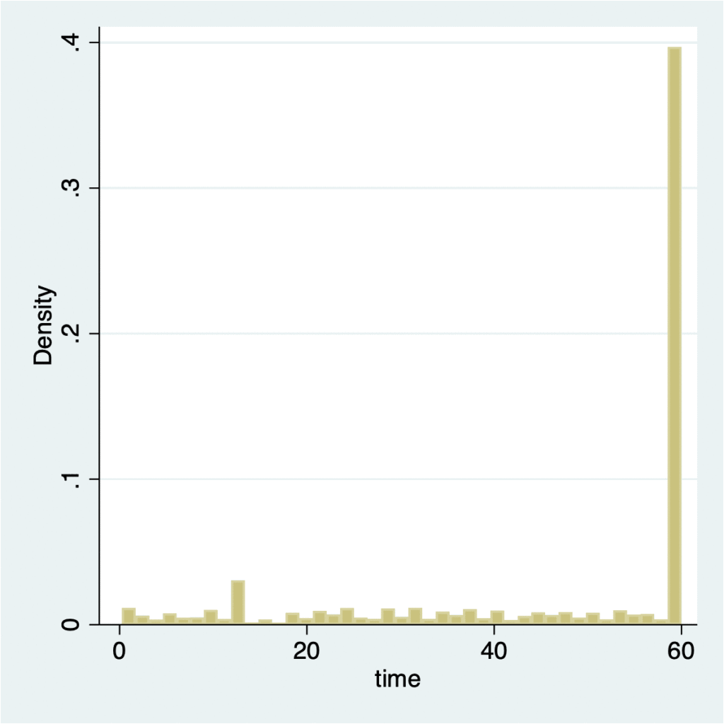
追跡期間time(月)を、0〜1未満、1〜6未満、6〜12未満、12〜24未満、24〜60のカテゴリに区分したdiscrete変数を作成します。
. egen discrete = cut(time), at(0 1 6 12 24 61) icodes

. table discrete, contents(min time max time)

----------------------------------
 discrete |  min(time)   max(time)
----------+-----------------------
        0 |        .25         .25
        1 |          1           5
        2 |          6          11
        3 |         12          23
        4 |         24          60
----------------------------------
discrete 0〜4を1〜5に変換します。
. replace discrete = discrete + 1
(3,120 real changes made)
ltableコマンドを使って、discrete別に生存率を算出します。noadjustオプションを利用すると、Kaplan-Meier法による生存率が出力されるので、便利です。
. ltable discrete death, noadjust

                 Beg.                                 Std.
   Interval     Total   Deaths   Lost    Survival    Error     [95% Conf. Int.]
-------------------------------------------------------------------------------
    1     2      3120      109      9     0.9651    0.0033     0.9580    0.9710
    2     3      3002       92     94     0.9355    0.0044     0.9263    0.9436
    3     4      2816       66    126     0.9136    0.0051     0.9031    0.9230
    4     5      2624       94    238     0.8808    0.0059     0.8687    0.8919
    5     6      2292       42   2250     0.8647    0.0063     0.8518    0.8765
-------------------------------------------------------------------------------
expand変数を使って、追跡期間(discrete)の分だけレコードを複製します。
. list momid kidid time discrete death if momid==2, clean

        momid   kidid   time   discrete   death
   5.       2     201     60          5       0
   6.       2     202     12          4       1
   7.       2     203     60          5       0
   8.       2     204      1          2       1

. expand discrete
(10,734 observations created)

. sort momid kidid

. list momid kidid time discrete death if momid==2, clean

         momid   kidid   time   discrete   death
   21.       2     201     60          5       0
   22.       2     201     60          5       0
   23.       2     201     60          5       0
   24.       2     201     60          5       0
   25.       2     201     60          5       0
   26.       2     202     12          4       1
   27.       2     202     12          4       1
   28.       2     202     12          4       1
   29.       2     202     12          4       1
   30.       2     203     60          5       0
   31.       2     203     60          5       0
   32.       2     203     60          5       0
   33.       2     203     60          5       0
   34.       2     203     60          5       0
   35.       2     204      1          2       1
   36.       2     204      1          2       1
同一kididのレコードに、連番の変数(interval)を追加します。
. bysort kidid: generate interval = _n

. list momid kidid time discrete interval death if momid==2, clean

         momid   kidid   time   discrete   interval   death
   21.       2     201     60          5          1       0
   22.       2     201     60          5          2       0
   23.       2     201     60          5          3       0
   24.       2     201     60          5          4       0
   25.       2     201     60          5          5       0
   26.       2     202     12          4          1       1
   27.       2     202     12          4          2       1
   28.       2     202     12          4          3       1
   29.       2     202     12          4          4       1
   30.       2     203     60          5          1       0
   31.       2     203     60          5          2       0
   32.       2     203     60          5          3       0
   33.       2     203     60          5          4       0
   34.       2     203     60          5          5       0
   35.       2     204      1          2          1       1
   36.       2     204      1          2          2       1
従属変数y=0を作成します。最終追跡時(discrete == interval)ではy=deathに設定します。
. generate y = 0

. replace y = death if interval == discrete
(403 real changes made)

. list momid kidid discrete interval death y if momid==2, clean

         momid   kidid   discrete   interval   death   y
   21.       2     201          5          1       0   0
   22.       2     201          5          2       0   0
   23.       2     201          5          3       0   0
   24.       2     201          5          4       0   0
   25.       2     201          5          5       0   0
   26.       2     202          4          1       1   0
   27.       2     202          4          2       1   0
   28.       2     202          4          3       1   0
   29.       2     202          4          4       1   1
   30.       2     203          5          1       0   0
   31.       2     203          5          2       0   0
   32.       2     203          5          3       0   0
   33.       2     203          5          4       0   0
   34.       2     203          5          5       0   0
   35.       2     204          2          1       1   0
   36.       2     204          2          2       1   1
これでdiscrete time hazard model用のデータセットがほぼ完成です。とりあえず、各intervalにおける死亡率を算出してみます。
. tabulate interval y, row

+----------------+
| Key            |
|----------------|
|   frequency    |
| row percentage |
+----------------+

           |           y
  interval |         0          1 |     Total
-----------+----------------------+----------
         1 |     3,011        109 |     3,120
           |     96.51       3.49 |    100.00
-----------+----------------------+----------
         2 |     2,910         92 |     3,002
           |     96.94       3.06 |    100.00
-----------+----------------------+----------
         3 |     2,750         66 |     2,816
           |     97.66       2.34 |    100.00
-----------+----------------------+----------
         4 |     2,530         94 |     2,624
           |     96.42       3.58 |    100.00
-----------+----------------------+----------
         5 |     2,250         42 |     2,292
           |     98.17       1.83 |    100.00
-----------+----------------------+----------
     Total |    13,451        403 |    13,854
           |     97.09       2.91 |    100.00
Complementary log-log modelを作成するためには、intervalのダミー変数を作成する必要があります。tabulate, generate()で作成します。
. tabulate interval, generate(int)

   interval |      Freq.     Percent        Cum.
------------+-----------------------------------
          1 |      3,120       22.52       22.52
          2 |      3,002       21.67       44.19
          3 |      2,816       20.33       64.52
          4 |      2,624       18.94       83.46
          5 |      2,292       16.54      100.00
------------+-----------------------------------
      Total |     13,854      100.00

. list momid kidid interval int1-int5 death y if momid==2, clean

         momid   kidid   interval   int1   int2   int3   int4   int5   death   y
   21.       2     201          1      1      0      0      0      0       0   0
   22.       2     201          2      0      1      0      0      0       0   0
   23.       2     201          3      0      0      1      0      0       0   0
   24.       2     201          4      0      0      0      1      0       0   0
   25.       2     201          5      0      0      0      0      1       0   0
   26.       2     202          1      1      0      0      0      0       1   0
   27.       2     202          2      0      1      0      0      0       1   0
   28.       2     202          3      0      0      1      0      0       1   0
   29.       2     202          4      0      0      0      1      0       1   1
   30.       2     203          1      1      0      0      0      0       0   0
   31.       2     203          2      0      1      0      0      0       0   0
   32.       2     203          3      0      0      1      0      0       0   0
   33.       2     203          4      0      0      0      1      0       0   0
   34.       2     203          5      0      0      0      0      1       0   0
   35.       2     204          1      1      0      0      0      0       1   0
   36.       2     204          2      0      1      0      0      0       1   1
Discrete time hazard model with complementary log-log model
cloglogコマンドを利用して、complementary log-logモデルを作成します。まずは暴露因子を含まないモデルを作成します。オプションに切片0およびハザード比表示を指定します。
. cloglog y int1-int5, noconstant eform

Iteration 0:   log likelihood = -1811.7312
Iteration 1:   log likelihood = -1811.6791
Iteration 2:   log likelihood = -1811.6791

Complementary log-log regression                Number of obs     =     13,854
                                                Zero outcomes     =     13,451
                                                Nonzero outcomes  =        403

                                                Wald chi2(5)      =    4943.80
Log likelihood = -1811.6791                     Prob > chi2       =     0.0000

------------------------------------------------------------------------------
           y |     exp(b)   Std. Err.      z    P>|z|     [95% Conf. Interval]
-------------+----------------------------------------------------------------
        int1 |   .0355608   .0034063   -34.83   0.000     .0294738    .0429048
        int2 |   .0311257   .0032452   -33.28   0.000      .025373    .0381826
        int3 |   .0237165   .0029194   -30.40   0.000     .0186326    .0301876
        int4 |   .0364806   .0037629   -32.10   0.000     .0298031    .0446541
        int5 |   .0184946   .0028538   -25.86   0.000     .0136678    .0250259
------------------------------------------------------------------------------
次に、年齢・性別補正モデルを作成します。
. cloglog y int1-int5 sex mage, noconstant eform

Iteration 0:   log likelihood =  -1811.344
Iteration 1:   log likelihood = -1811.2917
Iteration 2:   log likelihood = -1811.2917

Complementary log-log regression                Number of obs     =     13,854
                                                Zero outcomes     =     13,451
                                                Nonzero outcomes  =        403

                                                Wald chi2(7)      =    4941.87
Log likelihood = -1811.2917                     Prob > chi2       =     0.0000

------------------------------------------------------------------------------
           y |     exp(b)   Std. Err.      z    P>|z|     [95% Conf. Interval]
-------------+----------------------------------------------------------------
        int1 |   .0297238   .0067244   -15.54   0.000     .0190781    .0463097
        int2 |   .0260221   .0059782   -15.88   0.000     .0165879    .0408218
        int3 |   .0198284    .004736   -16.41   0.000     .0124158    .0316663
        int4 |   .0304998   .0069904   -15.23   0.000     .0194629    .0477956
        int5 |   .0154664   .0039604   -16.28   0.000     .0093633    .0255477
         sex |   1.026905   .1024613     0.27   0.790     .8445013    1.248707
        mage |    1.00634   .0076432     0.83   0.405     .9914704    1.021432
------------------------------------------------------------------------------
母親によるクラスターであると考えれば、Stataではvec(cluster cluster_var)オプションを利用して、robust standard error for clustered dataを求めることができます。
. cloglog y int1-int5 sex mage, noconstant eform vce(cluster momid)

Iteration 0:   log pseudolikelihood =  -1811.344
Iteration 1:   log pseudolikelihood = -1811.2917
Iteration 2:   log pseudolikelihood = -1811.2917

Complementary log-log regression                Number of obs     =     13,854
                                                Zero outcomes     =     13,451
                                                Nonzero outcomes  =        403

                                                Wald chi2(7)      =    4328.62
Log pseudolikelihood = -1811.2917               Prob > chi2       =     0.0000

                                (Std. Err. adjusted for 851 clusters in momid)
------------------------------------------------------------------------------
             |               Robust
           y |     exp(b)   Std. Err.      z    P>|z|     [95% Conf. Interval]
-------------+----------------------------------------------------------------
        int1 |   .0297238    .007154   -14.61   0.000     .0185453    .0476403
        int2 |   .0260221   .0069143   -13.73   0.000     .0154586     .043804
        int3 |   .0198284   .0053308   -14.58   0.000      .011707    .0335837
        int4 |   .0304998   .0077332   -13.76   0.000     .0185557    .0501323
        int5 |   .0154664   .0043305   -14.89   0.000     .0089343    .0267745
         sex |   1.026905   .1055175     0.26   0.796     .8395895    1.256012
        mage |    1.00634   .0087612     0.73   0.468     .9893139    1.023659
------------------------------------------------------------------------------
母親をランダム変数として組み込んだ、random-interceptモデルを作成します。xtcloglogコマンドを利用します。
. xtcloglog y int1-int5 sex mage, noconstant eform i(momid)

Fitting comparison model:

Iteration 0:   log likelihood =  -1811.344
Iteration 1:   log likelihood = -1811.2917
Iteration 2:   log likelihood = -1811.2917

Fitting full model:

tau =  0.0     log likelihood = -1911.7661
tau =  0.1     log likelihood = -1893.1909
tau =  0.2     log likelihood = -1874.1809
tau =  0.3     log likelihood = -1856.4094
tau =  0.4     log likelihood = -1842.2824
tau =  0.5     log likelihood = -1834.7269
tau =  0.6     log likelihood = -1837.5067

Iteration 0:   log likelihood = -1841.9925
Iteration 1:   log likelihood = -1808.6147
Iteration 2:   log likelihood = -1806.9026
Iteration 3:   log likelihood = -1806.7965
Iteration 4:   log likelihood = -1806.7963
Iteration 5:   log likelihood = -1806.7963

Random-effects complementary log-log model      Number of obs     =     13,854
Group variable: momid                           Number of groups  =        851

Random effects u_i ~ Gaussian                   Obs per group:
                                                              min =          1
                                                              avg =       16.3
                                                              max =         40

Integration method: mvaghermite                 Integration pts.  =         12

                                                Wald chi2(7)      =    2450.04
Log likelihood  = -1806.7963                    Prob > chi2       =     0.0000

------------------------------------------------------------------------------
           y |     exp(b)   Std. Err.      z    P>|z|     [95% Conf. Interval]
-------------+----------------------------------------------------------------
        int1 |   .0277072   .0065873   -15.08   0.000     .0173869    .0441532
        int2 |   .0245443   .0059068   -15.40   0.000     .0153144    .0393369
        int3 |   .0188305    .004693   -15.94   0.000     .0115538    .0306903
        int4 |   .0291856   .0069987   -14.74   0.000     .0182411    .0466969
        int5 |   .0149082   .0039561   -15.85   0.000     .0088623    .0250786
         sex |   1.033765   .1049692     0.33   0.744     .8472088    1.261402
        mage |   1.003026   .0081413     0.37   0.710     .9871959    1.019111
-------------+----------------------------------------------------------------
    /lnsig2u |  -1.254711   .3784523                     -1.996464   -.5129578
-------------+----------------------------------------------------------------
     sigma_u |   .5340022   .1010472                      .3685305    .7737713
         rho |   .1477433   .0476529                      .0762683    .2668511
------------------------------------------------------------------------------
Note: Estimates are transformed only in the first equation.
LR test of rho=0: chibar2(01) = 8.99                   Prob >= chibar2 = 0.001
\ 最新情報をチェック /